Insights

A blog post by Fatih Ozturk.

At UrbanStat, before we start modeling, we review the initial data extensively. We believe preprocessing is one of the most important steps of machine learning modeling. Data sets we receive from our clients are usually sourced through multiple systems, and to be able to start modeling we usually need to join all these different data sets together.

There is no silver bullet in this process, however we will mention most important steps in our risk scoring algorithm:

1 – Check Operations:

• Drop Duplicates: When we receive the training data sets we usually see duplicate records. For example, in insurance companies, when there is an endorsement or update for a policy it’s possible for them to send policy information both before the change and after the change to database and this can result in multiple same rows in time.

For python users it’s really easy to drop duplicated rows in a dataframe.

Example code:

dataframe = dataframe.drop_duplicates()

• Drop Irrelevant Parts: When you get your datasets from sources, according to your modeling purpose, you should check if data has completely irrelevant parts in it. For example, if your purpose is predicting claim probability of a 1-year long policy and got your datasets from an insurance company, you might find some policies having 3 years lifetime. So, in order to have a self-consistent modeling project you have to discard those policies having a life time different than 1 year.

Example code:

dataframe = dataframe[dataframe[‘Policy_Duration’]== 1]

• Have Consistent Columns: For numerical columns, make sure that values of them are in same range. You can have a look at statistical values of these columns to catch unexpected trends or check histogram plot to see whether there is a strange spike / outlier/ bin in the plot. For example, the data provided by the client had ‘Year_Built’ column in it and it tells the time when the building was built. The column was obviously numeric and the values were like 1979, 1992 and so on.  By checking statistics of that feature we realized that there are some entries like ‘83’,’75’ in a considerable amounts. We had to fix that column since predictive models would take value of 83 as lower than any other properly-entered years (1965,1972..).

When it comes to categorical columns, especially those having not much unique values, it’s better to check their unique values to see whether columns contain strange words or typos. For example, a column might have both ‘Burglary’ and ‘burglary’ strings and both represents the same treat which is `Burglary`. So, if you don’t make both values same, this situation will probably lower your modeling performance. In order to avoid such simple problem, you can make all values of your categorical columns in lower cases. For other cases, you can also discard spaces or replace them with ‘_’.

2- Merging Multiple Datasets:

In real life, it’s uncommon to have one single data set for any objective. For example, most of insurance companies record their customers’ policy, coverage, and claims information separately. So, based on objective of a data analysis or machine learning modeling, you need to be able to merge these files by a unique column exists in each of them. Make sure that you have this key column and can make a proper joining operation.

3- Handling missing values:

Having a missing value-free data set is not always needed in machine learning models. For example if you use decision trees as model, they can handle missing values and leaving them as Null can give better performance time to time. However, for neural nets and logistic regression filling missing values is a must. So, when it comes to filling, you can treat them in two general ways.

• Categorical columns:
  • If you believe being missing carries a meaningful value for a feature, then you can simply fill missing values with ‘missing’ string or anything fancy you want. Otherwise, you can fill with most frequent value in that column.

• Numerical columns:
  • Fill with mean, median values of that column.
  • Fill with a value which is out of range of that column. (like 999999, -999999, 0)
  • Try to predict missing values by treating that column as target in a regression model.

There can be some important columns requiring more attention rather than just filling zeros and means. So, you need to be more careful as handling them. To make this clear, let me give you another example. As UrbanStat we experience missing values in Latitude and Longitude columns of client’s policy data sets. Those features are quite important for us because we join external risk data sets by these columns. When we find missing values in those columns, data is geocoded with their Address information by our data team and filled with correct Longitude and Latitude information.

Underlying reason for your validation failure or under-fitting model performance could be not cleaning your data set enough. These simple data cleaning steps could help you outperform your competitors.

To learn more and quickly leverage what we’ve already successfully deployed for our carrier partners contact us at [email protected].

A blog post by Matt Carstens

“Their tech is great, but what can we do with it?” Statements like these are commonplace among boardrooms discussing how an InsurTech vendor solution is viewed within the walls of a carrier. Even clearly defined use cases are put into a moratorium, or shelved permanently because the amount of energy needed to break the inertia of legacy processes and systems, is simply too great.

The winners in the InsurTech space will be those firms who are able to push their solutions into multi-departmental or multiple pain-points at once.  Solutions targeting a single pain point, regardless of its sophistication, are much more vulnerable to being viewed as targets from the carriers in-house teams and legacy vendors.

Because of this, UrbanStat didn’t create just an advanced underwriting analytics platform, but a full suite holistic one that ties in risk visualization, two-way APIs that communicate with the carriers ERP systems, and machine learning based risk prediction models ready-made for the future. Combining all of these enables real-time communication between each other that significantly improves the speed and accuracy of decision-makers, and their systems, outside of just underwriting, but also into actuarial and claims departments, agencies and brokers, and the C-suite leadership as a whole.

The value created is much more complex to build and quite difficult to implement in-house efficiently as it touches so many departments. UrbanStat provides a clear advantage as we have worked on more than what a single carrier can see in their own universe of data, but the insights and knowledge gained from working for years with multiple carrier “universes” with wide-ranging geographies, cat/non-cat perils, business lines, and policy/claim features for both current and future business needs.

So as new technologies continue to push their way into executive conversations, savvy InsurTech providers that understand a clearly defined multi-departmental (or multi-pain point) value proposition helps change the conversation from “their tech is great, but what do we do with it” to “their tech is great, it allows us to improve………and replace………..”. This empowers forward-thinking carriers to loosen the grip of those old legacy systems and take advantage of modern technologies and the opportunities they provide throughout their ecosystem.

To learn more and quickly leverage what we’ve already successfully deployed for our carrier partners contact us at [email protected].

A blog post by Fatih Ozturk.

Model ensembling is one of the most used methods in order to improve machine learning performances one step further. With ensembling, you can leverage many model predictions and get more accurate and less biased results.

There are many ensembling methods but we are going to review weighted average on this post.  For more information, you can have a quick look on this well-structured and detailed post.

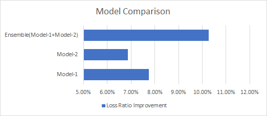
For comparison purposes, we will train two different models on an insurance policy/claim dataset, and model performance will be evaluated based on loss ratio improvement of the validation folds after we reject around ~7% of policyholders.

Modeling

For our current dataset, we are trying to predict how much risk (likelihood of a claim) a policyholder carries so that underwriters can reject those having high risks during risk selection process. Hence, we train our models on training data and score what would have happened to the loss ratio if we have rejected some policies in validation datasets. After getting predictions and rejecting high-risk policies, we monitor how loss ratio changes for multiple validation folds.

Both models are constructed with Light GBM (LGBM) which is a quite fast learner using gradient boosting decision trees. For more information about the algorithm, you can check this paper.

Although both models are trained with LGBM, they are quite different in terms of learning parameters. So, in the end, we have two completely different models.

Model – 1

Parameters:

• ‘learning_rate’: 0.1
• ‘max_depth’: -1
• ‘max_bin’: 10
• ‘objective’: ‘regression’
• ‘feature_fraction’: 0.5
• ‘num_leaves’:50
• ‘lambda_l1’: 0.1
• ‘min_data’: 650

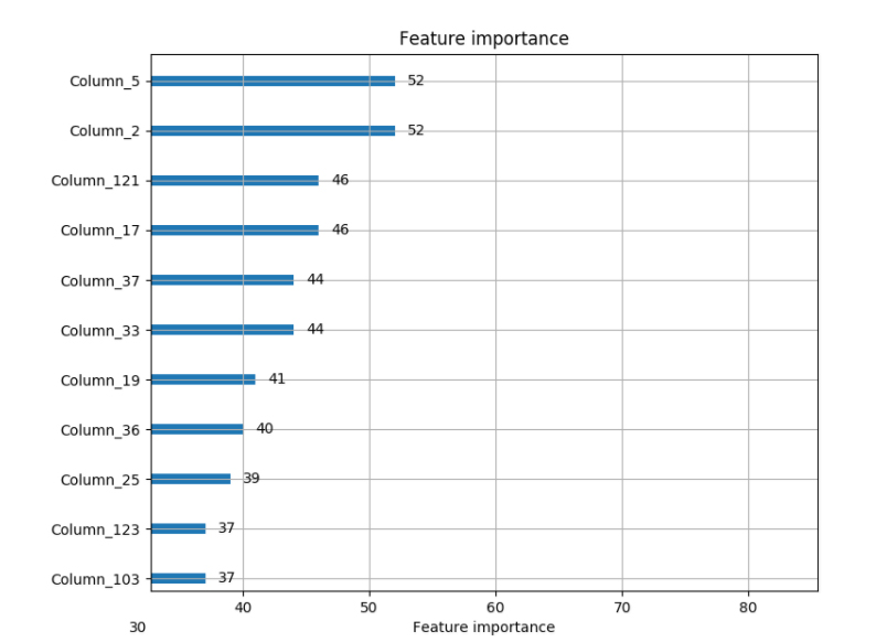
Feature Importance Plot: After running Model-1 we have listed most important features. The following figure sorts the features based on their importance:

Loss Ratio Improvement:

Decreased by 7.76% of current loss ratio at a reject ratio of 7%.

Model – 2

Parameters:

• ‘learning_rate’: 0.2
• ‘max_depth’: -1
• ‘max_bin’: 255
• ‘bagging_freq’ = 1,
• ‘objective’: ‘regression’
• ‘feature_fraction’: 0.5
• ‘num_leaves’:128
• ‘lambda_l1’: 1
• ‘min_data’: 20

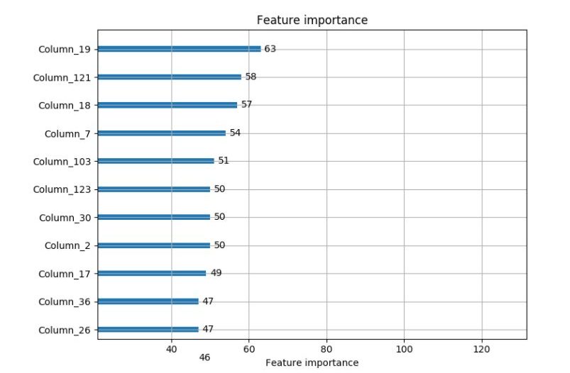
Feature Importance Plot: After running Model-2 we have listed most important features. The following figure sorts the features based on their importance:

Loss Ratio Improvement:

Decreased by  6.87% of current loss ratio at a reject ratio of 6.5%

Blending Predictions

Before blending different model predictions, there are some preprocess steps need to be checked.

Preprocess

For blending different predictions, we’ll use a simple weighted average. But before averaging them, there are some points that need to be considered. At first, predictions of the first model have come in the range of (0.000048 – 0.000891); however, the predictions of the second one are in a range o (0.0082 – 0.5622). Thus, if we do apply averaging without standardizing those predictions into the same scale, it’s highly expected that the order of the second model predictions won’t be affected by the operation.

Standardization can be applied by using the minimum and maximum value of the sets and the following formula.

min = prediction_list.min()

max = prediction_list.max()

prediction_list = (prediction_list – min) / (max – min)

After applying steps above, we’ve obtained two different prediction sets having quite similar ranges. Moreover, we’ve applied the same standardization onto validation folds by using training min and max values as well in order to avoid the potential leaks.

Another point that we need to consider is the correlation between those predictions. The lower the correlation, the higher the blending improvement. Let’s check mean correlation of each validation fold predictions.

In[40]: np.mean(correlation_list)

Out[40]: 0.5783084323078838

It’s ~0.58, which is great because it’s a quite low correlation for two different models even they provide an approximately same result. This means, there is still room to improve loss ratio by leveraging both predictions as both models were better at predicting different parts of the data.

Taking Weighted Average

Taking weighted average can be done by using following formula:

Weight = 0.5

blended_predictions = Weight*predictions_1+ (1 – Weight)*predictions_2

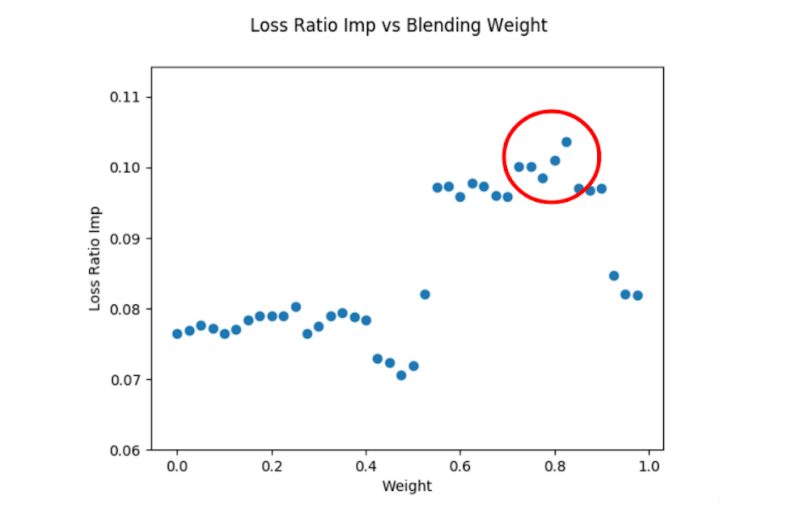
Also, you can change the weight manually and see the direction in which results change. Thanks to a “for loop”, you can generate weight values between 0 and 1 and you can simply find the weight in which the result is optimized.

As you can see on the scatter plot above, our loss ratio improvement is maximized at around 0.80 weight.

Results

With Weight = 0.7

Loss Ratio Improvement = 9.53% decrease at a reject ratio of 6.8%.

With Weight = 0.9

Loss Ratio Improvement = 9.75% decrease at a reject ratio of 6.9%.

With Weight = 0.83

Loss Ratio Improvement = 10.26% decrease at a reject ratio of 7%.

Conclusion

As you can see in the feature importance figures above, top features used during modeling are quite different from each other. Moreover, we had two different model predictions having a low correlation between them and they provided nearly same loss ratio improvement on their own. All these three statements are the sign of an upcoming improvement after ensembling.

We practiced simple weighted average on same validation predictions and obtained a significant loss ratio improvement by simply blending them. For future work, stacking can be tried as another ensembling method.

To learn more and quickly leverage what we’ve already successfully deployed for our carrier partners contact us at [email protected].

A blog post by Lal Kazdal.

In the first week of January 2018, East Coast battled with a colossal bomb cyclone that affected more than 100 million people (ABC News). Passing the southern states such as Florida, Georgia and South Carolina first, Storm Grayson stretched up to Maine, spanning 15 different states and 1,400 miles (PYMNTS.com). A storm is identified as a “bomb cyclone” if its pressure falls 24 millibars in 24 hours. Storm Grayson’s pressure fell 53 millibars in just 21 hours, making it one of the most explosive East Coast storms (Berman). The storm intensified on January 4 and in two days 5,000 flights were cancelled, 100,000 homes and businesses lost heat and power, numerous school districts closed, public transportation was disrupted and 22 people lost their lives (Samenow). Tallahassee, Florida saw snow for the first time in almost three decades as iguanas, stunned by the cold, fell from trees (Blinder, Alan, et al). UrbanStat tracked the storm closely and helped its partners with near-real time updates through live integration to NOAA’s radar services as seen below.

In the East Coast, Boston suffered the most, not only from 18 inches of snow, -20 degree wind-chills and 50 mile-an-hour winds, but also the worst flooding in four decades (Samuelson). The flooding was a result of the highest tide on record since 1978. The bomb cyclone struck Boston during supermoon when the tide is already higher than usual. With the strong wind, the tide gauge was a record of 15.16 feet, causing coastal floods (Finucane). During the storm, a subway station near the New England Aquarium was filled with ice chunks and storm surge. First-responders had to use rubber boats to evacuate people trapped in their cars and homes. Many residents of Plum Island, a barrier island about an hour away from Boston, had to be rescued by National Guards as the road connecting the island to the mainland became impassable.

Storm Grayson dissipated on January 6, leaving Bostoners in a hurry to fix their frozen and broken pipes (Berman). Analysts expect the claims for coastal flooding to surpass those for snow-related damage exact numbers to be published upcoming months.

To learn more and quickly leverage what we’ve already successfully deployed for our carrier partners contact us at [email protected].

Works Cited

• Berman, Mark. “A ‘Bomb Cyclone’ Slammed the East Coast with Snow and Ice. Now Comes the ‘Arctic Outbreak.’.” The Washington Post, 5 Jan. 2018, www.washingtonpost.com/news/post-nation/wp/2018/01/05/a-bomb-cyclone-slammed-the-east-coast-with-snow-and-ice-now-comes-the-arctic-outbreak/?utm_term=.cb619f6b34a6.
• Blinder, Alan, et al. “’Bomb Cyclone’: Snow and Bitter Cold Blast the Northeast.” The New York Times, 4 Jan. 2018, www.nytimes.com/2018/01/04/us/winter-snow-bomb-cyclone.html.
• “Bomb Cyclone Leaves Energy, Retail Exposed.” PYMNTS.com, 5 Jan. 2018, www.pymnts.com/news/retail/2018/bomb-cyclone-winter-snow-storm/.
• Buell, Spencer. “‘Bomb Cyclone’ Brought Flood of Ice and Slush to Boston.” Boston Magazine, 4 Jan. 2018, www.bostonmagazine.com/news/2018/01/04/boston-flooding-bomb-cyclone-2018/.
• Finucane, Martin. “It’s Official: Boston Breaks Tide Record – The Boston Globe.” BostonGlobe.com, 5 Jan. 2018, www.bostonglobe.com/metro/2018/01/05/official-boston-breaks-tide-record/UPbwDxgF0QXNOWvB9bcQ7L/story.html.
• “Frozen Iguanas Falling from Trees during Cold Snap in Florida.” CBS News, 5 Jan. 2018, www.cbsnews.com/news/florida-frozen-iguanas-falling-from-trees-during-cold-snap-bomb-cyclone-storm-east-coast/.
• “’Nobody Wants to Be Outside’: 100 Million People Affected by US Deep Freeze.” ABC News, 6 Jan. 2018, www.abc.net.au/news/2018-01-07/100-million-people-affected-by-us-east-coasts-deep-freeze/9309188.
• Samenow, Jason. “The ‘Bomb Cyclone’ by the Numbers: Here’s How Much Snow, Wind and Flooding It Unleashed.” The Washington Post, 5 Jan. 2018, www.washingtonpost.com/news/capital-weather-gang/wp/2018/01/05/the-bomb-cyclone-by-the-numbers-heres-how-much-snow-wind-and-flooding-it-unleashed/.
• Samuelson, Kate. “Snow Totals: Here’s How Much Snow the East Coast Got.” Time, 5 Jan. 2018, time.com/5089443/snow-totals-bomb-cyclone-east-coast/.